
Validation
Validation: Plate Fin Heat Sink
This validation case tests the Vanellus conjugate heat transfer solver on a plate-fin heat sink cooling a transistor under forced convection. We compare the results with measurements from Ventola et al. and a later SimScale OpenFOAM study.
The setup
This benchmark case represents one of the most common scenarios in electronics cooling: heat generated in an electronic component conducts into a heat sink, and is then removed by forced convection into the surrounding air.
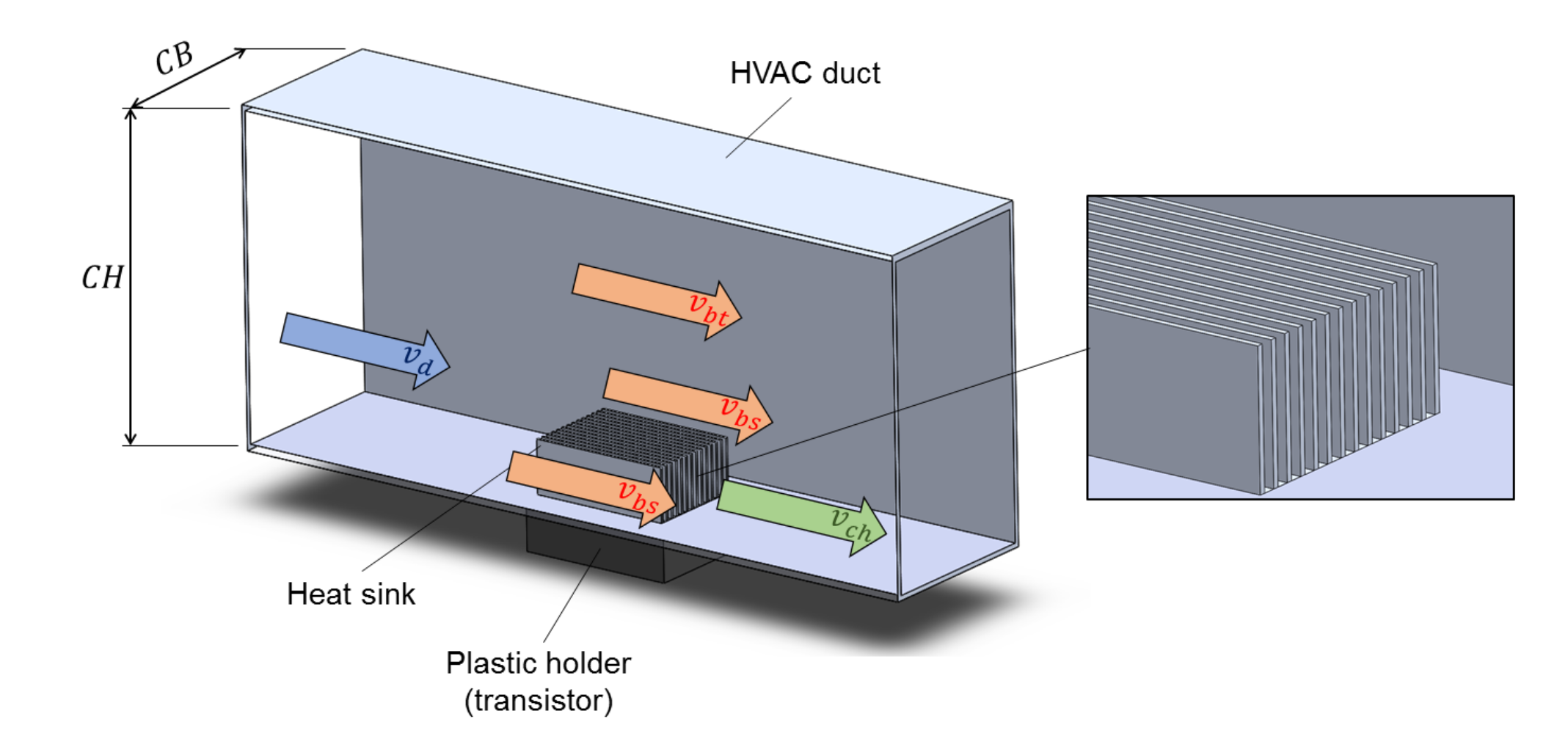
The case was originally presented by Ventola et al. (2016), and is pictured below. A MOSFET is placed in thermal contact with the bottom of an aluminum plate fin heat sink. The fins protrude into an HVAC duct, so the heat dissipated by the transistor enters the duct. Ambient air passes through the duct and over the fins.
Measurements
The experiments were designed to characterize the heat sink in a range of working conditions. Seven experiments were conducted, each with different flow rates, transistor powers and ambient temperatures.
The effectiveness of the heat sink is characterized by the thermal resistance along the path from the transistor to ambient air. This is defined as \(R_{ja} = (T_j - T_a) / P\), where \(T_j\) is the transistor junction temperature, \(T_a\) is the ambient air temperature, \(P\) is the applied power to the transistor, and \(R_{ja}\) is the junction-to-ambient resistance.
The junction temperature, \(T_j\), is found by measuring the temperature at the interface of the transistor and the heat sink, \(T_i\), and applying the junction-to-case resistance of \(R_{jc} = 0.5\,\mathrm{K/W}\) for the specific model of the transistor to get \(T_j = T_i + R_{jc}P\).
Results
For each of the seven experimental setups, we ran a steady-state conjugate heat transfer analysis using the \(k\)-\(\omega\) SST turbulence model. We discretized the domains using our rectilinear mesher, including both the air in the duct and the heat sink, with an applied heat flux boundary condition to model the transistor. We used the SIMPLE algorithm to iterate toward the steady-state, and stopped iterating once the measured junction temperature had converged.
We compared our results to both the experimental values in Ventola et al., and to a case study of the same problem conducted by SimScale. The SimScale study uses OpenFOAM and a tetrahedral mesh, while ours uses a rectilinear mesh. Both use the \(k\)-\(\omega\) SST turbulence model.
The plot below shows the results of our parameter study, alongside the experimental results and the simulation results from SimScale. The first plot shows the junction temperature of the transistor, and the second plot shows the calculated junction-to-ambient thermal resistance. Each data point represents a different flow rate, ambient temperature and transistor power, as presented in Table 2 of Ventola et al.
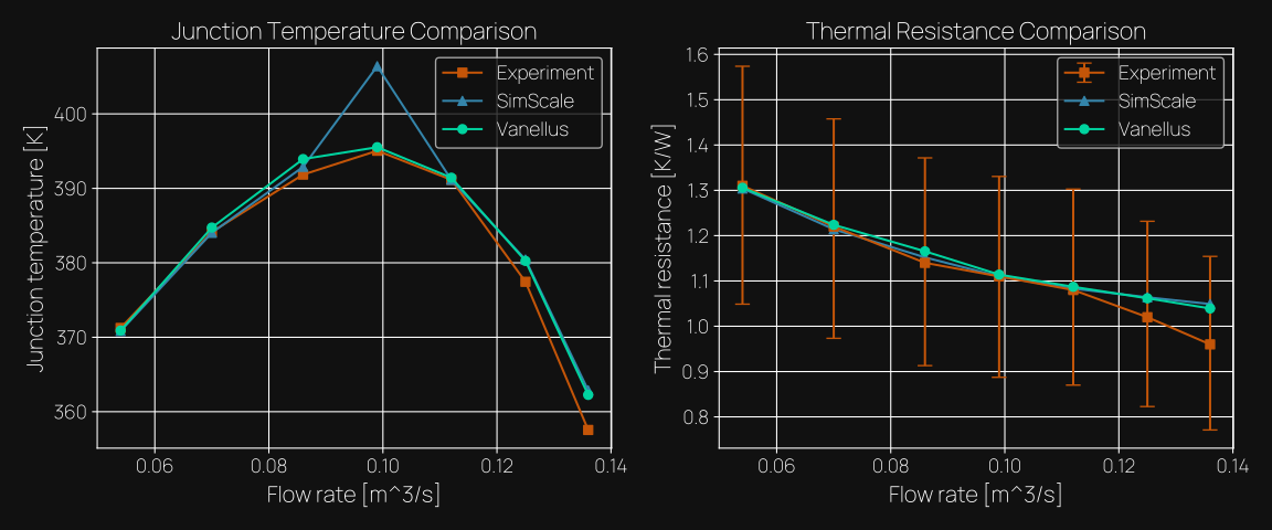
The results show the expected trend across the operating points. As flow rate increases, the thermal resistance decreases as the convective heat removal improves.
For the junction temperature, our results remain very close to the experimental values, and are much closer than the SimScale value for the \(0.099\,\mathrm{m^3\,s^{-1}}\) flow rate case.
For the thermal resistance results, all of the Vanellus results are well within the experimental margin of error, and are close to the results from SimScale.
To visualize the physics behind these numbers, below we show a snapshot of the velocity field for the \(0.125\,\mathrm{m^3\,s^{-1}}\) flow rate case, as well as the temperature field of the flow and heat sink.
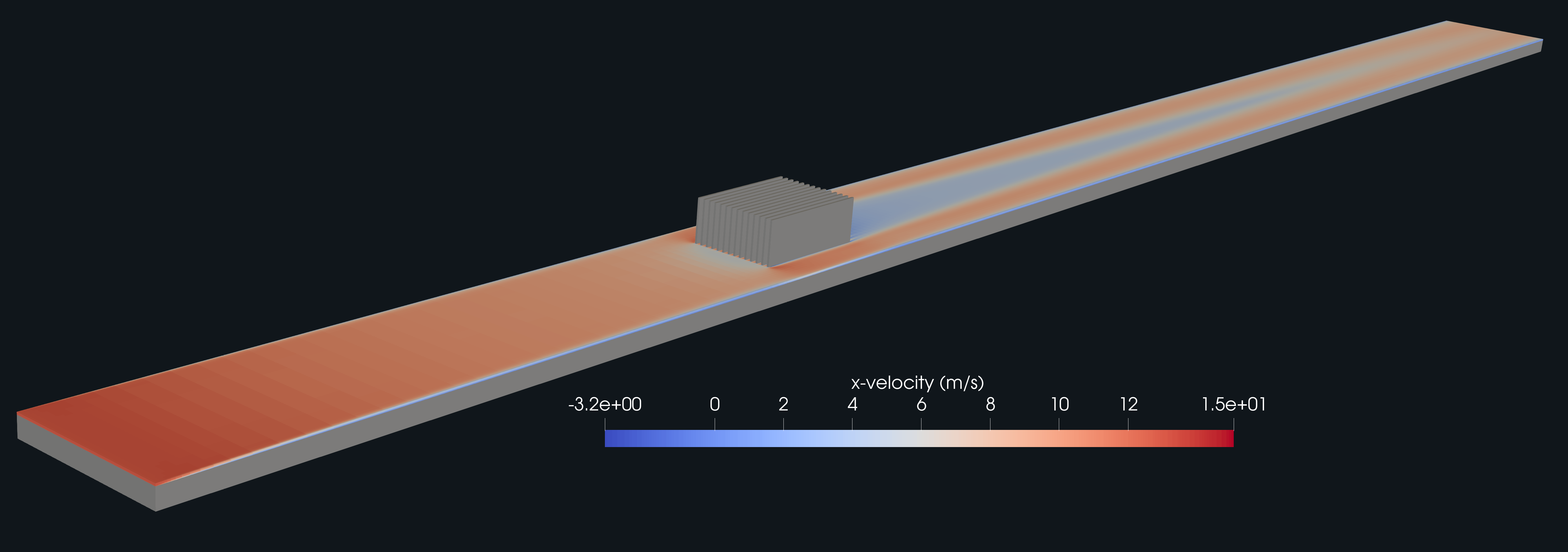
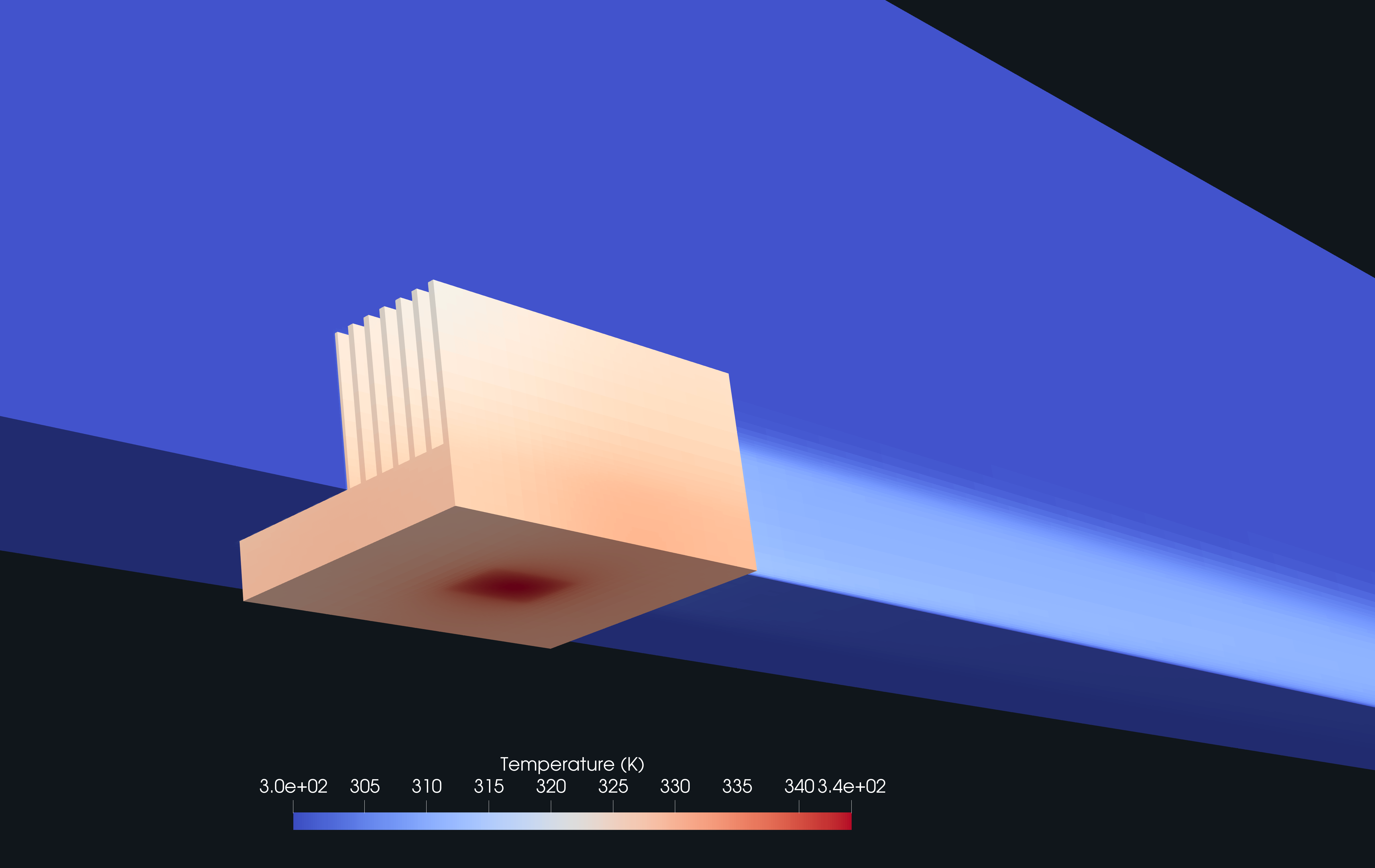
The velocity plot shows air passing through the fins and forming a large wake behind the heat sink. The temperature plot shows heat conducting from the base into the fins before convection carries it downstream.
Solver performance
For this benchmark, we used our in-house automated rectilinear meshing pipeline to generate meshes for each case. The meshes were refined near the fins of the heat sink to resolve the turbulent boundary layers. Although this meant remeshing for every case, each mesh took less than 0.1 seconds to generate.
The number of cells from each case varied from around 1.5 million to 2.5 million, increasing with the flow rate. The simulations were run until the junction temperature values converged, which required no more than 1000 iterations per case.
Running all seven cases in this parameter study one after another took under 8 minutes on an NVIDIA RTX Pro 6000 Blackwell GPU. In comparison, using traditional CPU-based CFD solvers, parameter studies of this size would be expected to take hours to complete.
Conclusion
Across all seven operating points, Vanellus remains close to the experimental junction temperatures and within the reported uncertainty for thermal resistance. Completing the study in under eight minutes demonstrates how GPU acceleration makes rapid operating-space exploration practical.
References
- Ventola, L.; Curcuruto, G.; Fasano, M.; Fotia, S.; Pugliese, V.; Chiavazzo, E.; Asinari, P. "Unshrouded Plate Fin Heat Sinks for Electronics Cooling: Validation of a Comprehensive Thermal Model and Cost Optimization in Semi-Active Configuration", Energies 2016, 9(8), 608. https://doi.org/10.3390/en9080608
- SimScale, "Conjugate Heat Transfer in Rectangular Fins", https://www.simscale.com/docs/validation-cases/conjugate-heat-transfer-rectangular-fins/